If you work with CSV files, you know how important it is to have a clear and consistent schema for your data. A schema defines your data’s structure, format, and types and helps you validate, transform, and analyze it. The problem is CSV files have no INFORMATION_SCHEMA or similar metadata store you can query to pull from. That’s why I wrote my file interrogator back in 2016. I needed a way to automatically infer the schema from the data by sampling it. I worked on this code until you could point it at any delimited file, and it would test each column to determine the narrowest data type that would fit all the values it had sampled for that column. It worked great! But like many projects that work, I sat them on the shelf and abandoned them.
It’s funny how we keep moving forward in technology but still face the same problems repeatedly. A colleague of mine was working with some CSV data in their Databricks instance and was struggling with extracting the data. I suggested it was time to update the file interrogator to Python to get through the problem. Luckily, before investing time in a rewrite, I searched Git Hub. I found https://github.com/capitalone/DataProfiler
The demo they shared seemed to be what I was looking for!

So I dug in to learn more.
Installing the library
Installing the library was simple. From a local PySpark or Databricks notebook, I can get the latest version from PyPi.
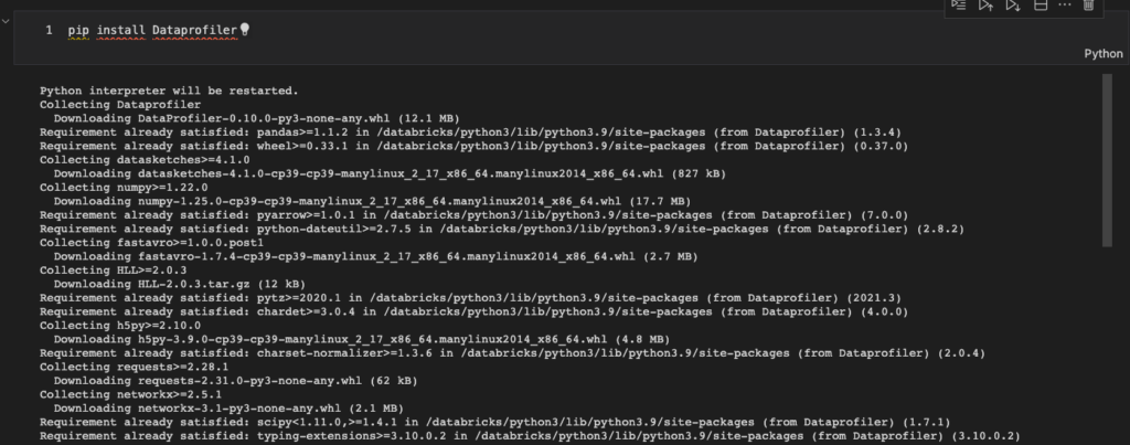
Once installed, I can import its functionality and get it to work. In this case, I also imported sql.types. You’ll see why shortly.

Our first demo
Now, grab a working CSV. If the CSV is malformed, the Capital One Data Profiler will fail. In my case, I downloaded a sample CSV from the internet, and it was malformed; it had a trailing double quote I had to remove to profile it.
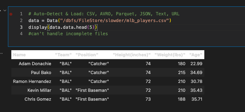
While you may think I’ve loaded the file’s contents into a data frame, beware, its type is a child type of the profiler. We’ll need to take more steps before creating a data frame for our file(s).

Profile the data
In our next step, we call the library to profile the file. Read through the documentation; you can get a lot of useful metadata using this profiler. We only need column names and data types, but you can get a lot more. You could even test for PII. That is a neat use case!
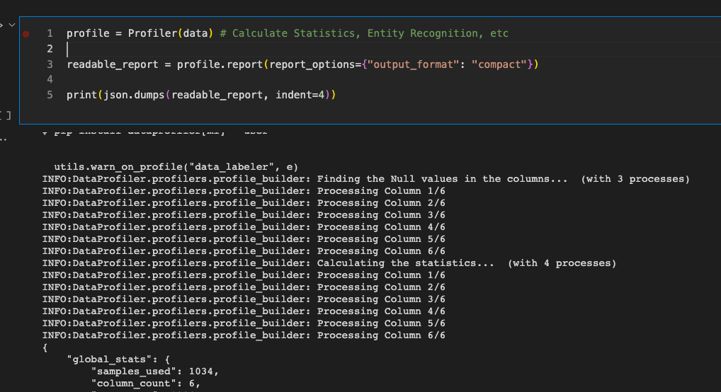
Let’s look at the readable report when we profile the mlb_player file.
{
"global_stats": {
"samples_used": 1034,
"column_count": 6,
"row_count": 1034,
"row_has_null_ratio": 0.0,
"row_is_null_ratio": 0.0,
"unique_row_ratio": 1.0,
"duplicate_row_count": 0,
"file_type": "csv",
"encoding": "utf-8",
"correlation_matrix": null,
"chi2_matrix": "[[nan, nan, nan, nan, nan, nan], ... , [nan, nan, nan, nan, nan, nan]]",
"profile_schema": {
"Name": [
0
],
" \"Team\"": [
1
],
" \"Position\"": [
2
],
" \"Height(inches)\"": [
3
],
" \"Weight(lbs)\"": [
4
],
" \"Age\"": [
5
]
},
"times": {
"row_stats": 0.0076
}
},
"data_stats": [
{
"column_name": "Name",
"data_type": "string",
"categorical": false,
"order": "random",
"samples": "['Chad Durbin', 'Vicente Padilla', 'Todd Linden', 'Robby Hammock',\n 'Aaron Rowand']",
"statistics": {
"min": 7.0,
"max": 19.0,
"mode": "[11.998]",
"median": 12.0006,
"sum": 12768.0,
"mean": 12.3482,
"variance": 3.9329,
"stddev": 1.9831,
"skewness": 0.3712,
"kurtosis": -0.0966,
"quantiles": {
"0": 11.0006,
"1": 12.0006,
"2": 13.9979
},
"median_abs_deviation": 1.008,
"vocab": "['M', 'F', 'x', 'i', 'r', ... , 's', 'N', 'v', 'C', \"'\"]",
"unique_count": 1032,
"unique_ratio": 0.9981,
"sample_size": 1034,
"null_count": 0,
"null_types": [],
"data_type_representation": {
"datetime": 0.0,
"int": 0.0,
"float": 0.0,
"string": 1.0
}
}
},
{
"column_name": " \"Team\"",
"data_type": "string",
"categorical": true,
"order": "random",
"samples": "[' \"HOU\"', ' \"CWS\"', ' \"BOS\"', ' \"HOU\"', ' \"ATL\"']",
"statistics": {
"min": 5.0,
"max": 6.0,
"mode": "[5.9995]",
"median": 5.9994,
"sum": 6036.0,
"mean": 5.8375,
"variance": 0.1362,
"stddev": 0.3691,
"skewness": -1.8326,
"kurtosis": 1.3611,
"quantiles": {
"0": 5.9991,
"1": 5.9994,
"2": 5.9997
},
"median_abs_deviation": 0.0003,
"vocab": "['I', 'L', 'M', 'F', 'Y', ... , 'N', 'B', 'U', 'C', 'A']",
"unique_count": 30,
"unique_ratio": 0.029,
"categories": "[' \"NYM\"', ' \"ATL\"', ' \"OAK\"', ... , ' \"FLA\"', ' \"STL\"', ' \"ARZ\"']",
"gini_impurity": 0.9666,
"unalikeability": 0.9675,
"categorical_count": {
" \"NYM\"": 38,
" \"ATL\"": 37,
" \"OAK\"": 37,
" \"DET\"": 37,
" \"CHC\"": 36,
" \"BOS\"": 36,
" \"WAS\"": 36,
" \"PHI\"": 36,
" \"CIN\"": 36,
" \"PIT\"": 35,
" \"MLW\"": 35,
" \"COL\"": 35,
" \"BAL\"": 35,
" \"ANA\"": 35,
" \"CLE\"": 35,
" \"TEX\"": 35,
" \"KC\"": 35,
" \"HOU\"": 34,
" \"SEA\"": 34,
" \"SF\"": 34,
" \"TOR\"": 34,
" \"SD\"": 33,
" \"MIN\"": 33,
" \"LA\"": 33,
" \"TB\"": 33,
" \"CWS\"": 33,
" \"NYY\"": 32,
" \"FLA\"": 32,
" \"STL\"": 32,
" \"ARZ\"": 28
},
"sample_size": 1034,
"null_count": 0,
"null_types": [],
"data_type_representation": {
"datetime": 0.0,
"int": 0.0,
"float": 0.0,
"string": 1.0
}
}
},
{
"column_name": " \"Position\"",
"data_type": "string",
"categorical": true,
"order": "random",
"samples": "[' \"Starting Pitcher\"', ' \"Third Baseman\"', ' \"Catcher\"', ' \"Catcher\"',\n ' \"Outfielder\"']",
"statistics": {
"min": 10.0,
"max": 20.0,
"mode": "[17.005]",
"median": 17.0025,
"sum": 16406.0,
"mean": 15.8665,
"variance": 7.6918,
"stddev": 2.7734,
"skewness": -0.6505,
"kurtosis": -0.6731,
"quantiles": {
"0": 13.0067,
"1": 17.0025,
"2": 17.0095
},
"median_abs_deviation": 1.9994,
"vocab": "['F', 'o', 'r', 'i', 'a', ... , 't', 'P', 's', 'B', 'C']",
"unique_count": 9,
"unique_ratio": 0.0087,
"categories": "[' \"Relief Pitcher\"', ... , ' \"Designated Hitter\"']",
"gini_impurity": 0.8102,
"unalikeability": 0.811,
"categorical_count": {
" \"Relief Pitcher\"": 315,
" \"Starting Pitcher\"": 221,
" \"Outfielder\"": 194,
" \"Catcher\"": 76,
" \"Second Baseman\"": 58,
" \"First Baseman\"": 55,
" \"Shortstop\"": 52,
" \"Third Baseman\"": 45,
" \"Designated Hitter\"": 18
},
"sample_size": 1034,
"null_count": 0,
"null_types": [],
"data_type_representation": {
"datetime": 0.0,
"int": 0.0,
"float": 0.0,
"string": 1.0
}
}
},
{
"column_name": " \"Height(inches)\"",
"data_type": "int",
"categorical": true,
"order": "random",
"samples": "[' 73', ' 73', ' 70', ' 74', ' 76']",
"statistics": {
"min": 67.0,
"max": 83.0,
"mode": "[74.]",
"median": 73.9947,
"sum": 76203.0,
"mean": 73.6973,
"variance": 5.3168,
"stddev": 2.3058,
"skewness": 0.2254,
"kurtosis": 0.3466,
"quantiles": {
"0": 72.0014,
"1": 73.9947,
"2": 75.0113
},
"median_abs_deviation": 1.9882,
"num_zeros": 0,
"num_negatives": 0,
"unique_count": 17,
"unique_ratio": 0.0164,
"categories": "[' 74', ' 73', ' 75', ' 72', ... , ' 81', ' 82', ' 67', ' 83']",
"gini_impurity": 0.8755,
"unalikeability": 0.8764,
"categorical_count": {
" 74": 175,
" 73": 167,
" 75": 160,
" 72": 152,
" 76": 103,
" 71": 89,
" 77": 57,
" 70": 52,
" 78": 27,
" 69": 19,
" 79": 14,
" 68": 7,
" 80": 5,
" 81": 2,
" 82": 2,
" 67": 2,
" 83": 1
},
"sample_size": 1034,
"null_count": 0,
"null_types": [],
"data_type_representation": {
"datetime": 0.0,
"int": 1.0,
"float": 1.0,
"string": 1.0
}
}
},
{
"column_name": " \"Weight(lbs)\"",
"data_type": "string",
"categorical": true,
"order": "random",
"samples": "[' 185', ' 215', ' 231', ' 175', ' 240']",
"statistics": {
"min": 3.0,
"max": 4.0,
"mode": "[3.9995]",
"median": 3.9995,
"sum": 4135.0,
"mean": 3.999,
"variance": 0.001,
"stddev": 0.0311,
"skewness": -32.1559,
"kurtosis": 1034.0,
"quantiles": {
"0": 3.9992,
"1": 3.9995,
"2": 3.9997
},
"median_abs_deviation": 0.0003,
"vocab": "['5', '3', '2', '7', '0', ... , '1', '8', '9', ' ', '6']",
"unique_count": 90,
"unique_ratio": 0.087,
"categories": "[' 200', ' 190', ' 180', ... , ' 270', ' 182', ' 163']",
"gini_impurity": 0.95,
"unalikeability": 0.9509,
"categorical_count": {
" 200": 108,
" 190": 97,
" 180": 81,
" 210": 72,
" 220": 72,
" 205": 55,
" 185": 52,
" 195": 48,
" 170": 40,
" 215": 39,
" 230": 33,
" 175": 25,
" 225": 24,
" 240": 20,
" 160": 15,
" 235": 13,
" 208": 11,
" 250": 10,
" 192": 9,
" 165": 9,
" 188": 9,
" 219": 8,
" 245": 8,
" 197": 8,
" 206": 7,
" 202": 7,
" 211": 6,
" 212": 6,
" 198": 5,
" 224": 5,
" 222": 5,
" 228": 5,
" 209": 5,
" 150": 4,
" 184": 4,
" 204": 4,
" 176": 4,
" 260": 4,
" 231": 4,
" 186": 4,
" 223": 4,
" 196": 3,
" 177": 3,
" 193": 3,
" 187": 3,
" 167": 3,
" 203": 3,
" 189": 3,
" 194": 3,
" 201": 3,
" 244": 3,
" 207": 3,
" 155": 3,
" 237": 2,
" 199": 2,
" 191": 2,
" 221": 2,
" 213": 2,
" 226": 2,
" 232": 2,
" 178": 2,
" 218": 2,
" 234": 2,
" 216": 2,
" 229": 2,
" 156": 1,
" 168": 1,
" \"\"": 1,
" 246": 1,
" 217": 1,
" 183": 1,
" 257": 1,
" 238": 1,
" 254": 1,
" 239": 1,
" 290": 1,
" 255": 1,
" 164": 1,
" 249": 1,
" 275": 1,
" 227": 1,
" 181": 1,
" 214": 1,
" 172": 1,
" 278": 1,
" 241": 1,
" 233": 1,
" 270": 1,
" 182": 1,
" 163": 1
},
"sample_size": 1034,
"null_count": 0,
"null_types": [],
"data_type_representation": {
"datetime": 0.0,
"int": 0.999,
"float": 0.999,
"string": 1.0
}
}
},
{
"column_name": " \"Age\"",
"data_type": "float",
"categorical": false,
"order": "random",
"samples": "[' 25.25', ' 24.51', ' 24.96', ' 24.25', ' 27.47']",
"statistics": {
"min": 20.9,
"max": 48.52,
"mode": "[24.94633]",
"median": 27.9224,
"sum": 29713.76,
"mean": 28.7367,
"variance": 18.6651,
"stddev": 4.3203,
"skewness": 0.8601,
"kurtosis": 0.5502,
"quantiles": {
"0": 25.4412,
"1": 27.9224,
"2": 31.2437
},
"median_abs_deviation": 2.7906,
"num_zeros": 0,
"num_negatives": 0,
"precision": {
"min": 1.0,
"max": 4.0,
"mean": 3.905,
"var": 0.1033,
"std": 0.3214,
"sample_size": 1034,
"margin_of_error": 0.0329,
"confidence_level": 0.999
},
"unique_count": 725,
"unique_ratio": 0.7012,
"sample_size": 1034,
"null_count": 0,
"null_types": [],
"data_type_representation": {
"datetime": 0.0,
"int": 0.0048,
"float": 1.0,
"string": 1.0
}
}
}
]
}Pull the data_stats array into a data frame.
The data_stats array contains both column names and data types. Let’s pull that into a data frame.
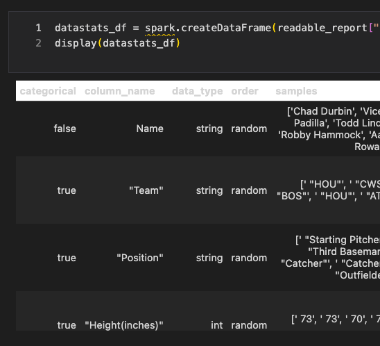
Now, let’s build a function that can take this data frame and return a schema we could then use to load that CSV data to a PySpark data frame.
def buildSchemaFromDataStats(df):
    schema = StructType([])

    for row in df.select("column_name", "data_type").collect():
        #clean up column_names
        column_name = row.column_name.replace('"','').replace(' ', '_')
        #re-init row_added each loop
        row_added = False
        #match doesn't start until python 3.10, so here's bunch of if statements
        #also, I only uncovered four datatypes in the library so far. Needs more testing
        if row.data_type == "datetime":
            schema = StructType([
                *schema.fields,
                StructField(column_name, TimestampType(), True)
            ])
            row_added = True
        if row.data_type == "float":
            schema = StructType([
                *schema.fields,
                StructField(column_name, FloatType(), True)
            ])
            row_added = True
        if row.data_type == "int":
            schema = StructType([
                *schema.fields,
                StructField(column_name, IntegerType(), True)
            ])
            row_added = True

        if row_added == False:
            #default to text
            schema = StructType([
                *schema.fields,
                StructField(column_name, StringType(), True)
            ])

    return schema
I set up an empty StructType that will hold my collection of columns. Then I run through each column_name and data_type in the data frame. I added a quick cleanup to the column names since I had some spaces and double quotes. This should be a separate function with all the logic for taking “raw” column names and creating Python-safe versions.
Next, I had to add several if-then statements since the current Databricks images run Python 3.9, and you can’t use match until 3.10. In reviewing the documentation and personal testing, I’ve only seen four data types returned from the Capital One Data Profiler. I would encourage additional testing to see if more are possible.
Finally, I return the schema to be used in our ETL notebooks.

Now that we have a PySpark schema let’s use it to read in our CSV data!
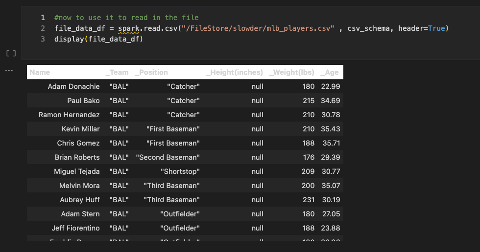
Check out the schema for our data frame.

Conclusion
You’ve just learned how to read your semi-structured data files using the Capital One Data Profiler. This tool can help you analyze and understand your data faster and easier. I encourage you to dig into this tool. Further, we’re only scratching the surface of how it can help! If you have any questions or feedback, please don’t hesitate to email me. I’d love to hear from you and help you get the most out of your data!